I've done route studies on builds across 14 states. And I'll tell you — the single most expensive mistake an ISP can make in the design phase isn't a bad splice plan or a miscounted strand count. It's defaulting to road-following when the data clearly supports a better path. Route miles drive everything: materials cost, labor hours, make-ready scope, permitting complexity, and construction timeline. Shave the miles and you shave the budget. It's that direct.
This article covers the fiber route optimization techniques we use on real projects — the GIS workflows, the infrastructure reuse strategies, the terrain scoring methods, and the ROW conflict filters that together make the difference between a build that comes in under budget and one that blows past its contingency reserve in week three. These aren't theoretical frameworks. They're the actual methods behind a $2.1M cost reduction on a BEAD project we completed last year.
Why Route Miles Are Costing You More Than You Think
Here's a number worth sitting with: $45–$62 per location passed. That's the all-in construction cost range we see on mid-complexity rural fiber builds — including materials, labor, make-ready, and permitting overhead. At that rate, one unnecessary route mile — say, 23 additional poles you didn't need — isn't just a materials problem. It's $80,000–$140,000 in construction cost that shouldn't be on the project at all.
The "obvious path" problem is real. Engineers under schedule pressure default to road-following because it's fast to design, easy to permit, and easy to explain in a meeting. Roads are pre-cleared corridors. They're politically legible. But on rural builds, roads don't go where your subscribers are — they go where roads go. A farm cluster that sits 0.7 miles off a county highway is accessible in a straight shot across an adjacent field easement. Following the road adds 1.6 miles and two curve transitions. That detour, multiplied across a 47-mile build, compounds fast.
On a project in southern Iowa last year — 2,400 locations across three counties — the initial road-following route came in at 47.6 miles. After a full GIS optimization pass, we found a 31.3-mile route. That's not an edge case or a lucky coincidence. It came from systematically applying the techniques below. The obvious path was 14.2 miles on one stretch alone; we found a 9.8-mile route using a combination of power line corridor access and two co-op trench agreements. The savings on that one stretch: roughly $400,000 in construction cost.
If your current route design process starts with "draw along the road," you're leaving money in the ground — literally.
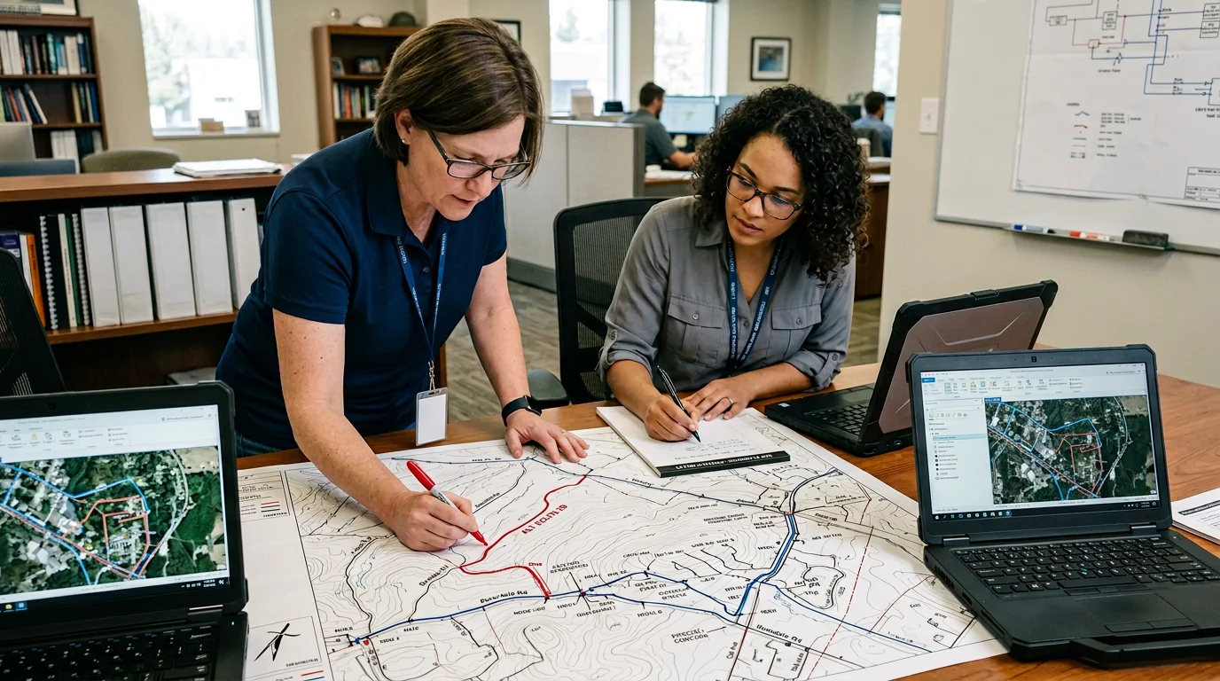
Start With Satellite and Aerial Imagery, Not the Map
The map — whether it's Google Maps or a county parcel basemap — shows roads, parcel lines, and labeled features. What it doesn't show is what's actually on the ground between those roads. That's where the route miles are hiding. And that's why every route study we do starts with satellite and aerial imagery, not a road layer.
Road-following adds 20–40% to route mileage on rural projects. That's not an estimate — it's what we see consistently when we compare optimized routes against initial road-following designs across the project types we work on. The difference is most dramatic in agricultural counties where road grids are sparse and parcels are large. A section of Indiana farmland that's 1 mile × 1 mile has a lot of interior space that a road-following route never touches efficiently.
Google Earth Pro and ArcGIS World Imagery are the two tools I use for initial visual scouting. The workflow is straightforward: drop parcel centroids on the imagery layer, identify natural corridors between demand clusters, and look for three specific things. First — existing utility corridors. Power transmission lines, natural gas pipelines, and electric distribution feeders are pre-surveyed, already have ROW established (or relationships that can get you there), and often run in near-straight paths across terrain that roads avoid. Second — terrain breaks. Ridgelines, drainages, and wetland complexes that a road route navigates around but a cross-country route can sometimes vault with a single bore or aerial crossing at the narrowest point. Third — developed parcel clusters. Groups of homes or businesses that share a common access point from a main road; a single distribution feed from that access point can serve all of them rather than a mile of road frontage serving them one by one.
What you're building in this phase is a candidate corridor list — three to five possible route paths that get from the serving node to the demand cluster with minimum deviation. You don't optimize here; you identify the options. The optimization happens in GIS.
Field note: On an eastern Kansas build, satellite imagery revealed a 6.2-mile stretch of rural electric co-op distribution line running almost exactly parallel to our target demand cluster — less than 400 feet off the parcel centroids we were trying to reach. The road route to the same cluster was 9.1 miles. We negotiated a joint-use agreement with the co-op in three weeks and lashed on existing strand. That single corridor identification saved the ISP $580,000 against the road-following design.
Reuse Existing Infrastructure First
Before you design a single foot of new infrastructure, you need to know what's already there. This isn't just good engineering — it's the highest-return cost reduction available on most builds. The cost difference between aerial lashing on existing strand and new underground conduit installation is $18–$65 per foot, depending on soil conditions, crossing requirements, and installation method. On a 5-mile segment, that's $475,000–$1.7M in potential cost avoidance if you can reuse what's there.
Start with call-before-you-dig records and work outward. 811 data gives you the locates picture, but for fiber route planning you need more — NRECA fiber maps (if you're working in rural electric co-op territory), CLEC records from the state PUC, and in BEAD project areas, the state broadband office's existing infrastructure layer. These sources combined tell you where aerial strand exists, where conduit has been placed, and where other carriers have already solved the ROW problem you're trying to solve.
Electric co-op partnerships deserve special attention. In rural areas — which is where most BEAD projects are — the local electric cooperative often has distribution infrastructure running exactly where you need fiber. Joint-use agreements for aerial attachment on co-op poles are negotiable, and co-ops are increasingly motivated to partner because broadband access is an explicit part of their mission in many states. Shared trench arrangements — where the co-op is doing underground work anyway and you ride their excavation — can reduce your underground installation cost to conduit materials plus splicing alone, with zero trenching cost.
For BEAD subgrantee HLD requirements, documenting reused infrastructure isn't optional — it's a compliance item. Program offices require that existing infrastructure included in your build be documented with source data, attachment agreements, and cost attribution. Getting that documentation right during the design phase, not after construction, is critical. Our HLD design services include infrastructure reuse documentation as a standard deliverable for BEAD projects specifically because of this requirement.
GIS-Based Route Scoring — How We Do It
Once candidate corridors are identified and existing infrastructure is mapped, the actual route optimization is a GIS exercise. Here's the workflow we use — it's not proprietary, and any ISP with an engineer who knows ArcGIS or QGIS can replicate it.
Start with three data layers: parcel centroids (your demand points), existing infrastructure (aerial strand, conduit, co-op poles), and a terrain DEM at 10-meter resolution or better. The DEM is critical — it's what lets you score routes by actual construction difficulty rather than distance alone.
The scoring formula we use assigns a cost to every raster cell in the study area:
(Route length × terrain factor) + crossing penalties + ROW conflict flags
Terrain factor scales from 1.0 (flat, well-drained) to 1.8 (slopes above 15%, unstable substrate). Crossing penalties assign a fixed cost to each water crossing or road bore — typically $12,000–$35,000 per crossing depending on width and crossing type. ROW conflict flags mark cells where permitting is known to be slow (railroad corridors, state highway ROW, federal land) with a time penalty expressed as cost.
With the cost surface built, least-cost path analysis in ArcGIS Network Analyst — or the equivalent r.cost/r.drain workflow in QGIS — finds the minimum-cost route between the serving node and each demand cluster. This isn't a single run; you typically iterate 4–6 times, adjusting the weighting between distance, terrain, and crossing penalties to see how sensitive the optimal route is to those assumptions.
Midpoint placement logic follows from the route output. Once you know where the route runs, you can identify distribution point locations that minimize total drop lengths to individual parcels. A distribution point placed at the geographic centroid of a cluster — rather than at the road frontage — can cut average drop length by 40–60%, which matters when you're talking 200 drops at $800–$1,400 per drop.
This is what GIS-driven route planning actually looks like in practice — not a static map layer, but an iterative scoring model that finds paths a road-following approach will never identify.
ROW Conflicts and Terrain Routing
The cost surface model handles ROW conflicts and terrain mathematically, but there are specific categories that need explicit judgment — not just a penalty number.
Railroads. Railroad crossing permits run 4–18 months depending on the railroad company and the type of crossing. If a route requires a railroad crossing and there's an alternative within 0.5 route miles, I'll almost always recommend the detour. The math is simple: 0.5 extra miles at $45/foot installed for aerial is about $118,800. A permit delay of 6 months — even assuming it doesn't hold up the entire project — easily costs more than that in carrying costs and schedule compression on the back end.
Water crossings. HDD (horizontal directional drilling) for a fiber crossing runs $85–$220 per foot depending on bore length, substrate, and casing requirements. A 200-foot bore across a creek costs $17,000–$44,000. A 400-foot bore across a river with rock substrate can hit $88,000. Always check LIDAR data to confirm water feature widths before assuming a crossing is minor — what looks like a seasonal drainage on a road map can be a 60-foot wetland complex that requires a full bore. For aerial vs. underground construction decisions at water crossings, aerial lashing above the water feature — where span length and clearance allow — is consistently cheaper than a bore.
Elevation and grade. Grades above 15% add 12–18% to trenching cost. That doesn't sound like much until you're talking about a 2.3-mile hillside segment where standard trenching would cost $680,000 and grade-adjusted cost is $800,000+. Routing around a ridge via a longer but flatter path often wins on total cost — and on construction timeline, since steep-grade work moves slower and carries higher safety overhead.
State highway ROW. Permit timelines for state highway ROW average 6–11 weeks in most states. County road ROW runs 1–3 weeks. Where a route can choose between a state highway crossing and a county road crossing of similar span length, the county road is almost always the better choice — you don't save 8 weeks of schedule to cross 40 fewer feet of asphalt. Field survey data accuracy at crossing points matters a lot here, because the permit submission requires precise bore location, casing specs, and depth — and you can't get those right from imagery alone.
The Real Cost Savings: A BEAD Project Example
Here's a real project. Rural ISP in the Midwest — I won't name the county because the grant application is still in review — 2,400 locations to pass across three counties. The project was initially designed by following the county road system, which is how most rural designs start.
Initial route: 47.6 miles.
We ran a full GIS optimization study. That included satellite imagery analysis to identify utility corridors, NRECA fiber map review to find existing strand, co-op engagement on two potential joint-use corridors, terrain DEM analysis to flag grade-sensitive segments, and four iterations of least-cost path modeling with different weighting schemes. We also identified a railroad crossing in the initial route that would have taken an estimated 7 months to permit — and found a county road crossing 0.4 miles south that avoided it entirely.
Optimized route: 31.3 miles.
That's a 34.2% reduction in route miles. The cost breakdown tells the story clearly:
| Factor | Initial Route | Optimized Route |
|---|---|---|
| Total route miles | 47.6 miles | 31.3 miles |
| Estimated construction cost | $6.8M | $4.7M |
| Cost reduction | — | $2.1M (30.9%) |
| Estimated construction timeline | ~38 weeks | ~24 weeks |
| Railroad crossings | 1 (7-month permit) | 0 |
| Reused infrastructure (aerial strand) | 0 miles | 8.4 miles |
The $2.1M reduction came from three sources roughly equally: 16.3 fewer miles of new construction, 8.4 miles of aerial attachment on existing co-op strand instead of new underground, and eliminating the railroad crossing that would have required both a bore and a 7-month permit window. The 14-week schedule reduction is, in many ways, worth as much as the cost reduction — shorter construction timelines mean faster service activation, faster revenue, and lower exposure to weather and supply-chain risk.
That's what middle-mile network design optimization looks like when it's done with real data rather than a road layer. And it's why the route study phase — which cost about $38,000 in engineering time — returned more than 55× its cost in construction savings.
For ISPs working on OSP engineering support for rural ISPs, having an outside team run this analysis is often the fastest path to getting it right. Internal teams are close to the project and under schedule pressure — the road-following route is always faster to produce in the short term. An outside engineering team running a structured GIS optimization study can challenge those defaults without the political overhead of contradicting internal decisions.
On BEAD compliance: The optimized route documentation we produced for this project — including the GIS cost surface, corridor scoring matrices, co-op agreement letters, and route comparison exhibits — became a core part of the subgrantee's technical submission. Program offices want to see that route decisions are defensible. A well-documented route optimization study is one of the strongest signals you can send that your project team knows what they're doing.